The Excel Conditional Formatting : Advanced
Have you ever wanted to color a cell by checking status of another cell and found it... not so simple ?
I read this excellent Excel 2003 article about conditional formatting , and decided to update it to the 2007 version of Excel.
Lets start with just a
 rudimentary worksheet about toDos and statuses
as you can see our statuses are "ok" and "not ok" (or nothing)
Next create a condition
 Now add a conditional formatting by selecting the rows you wish to color (not the rows to be tested!!)
In our case it's all of colums B and C so select'em
go to Conditional Formatting and select NEW RULE
a popup will open called New Formatting Rule.
Select the last option (Use formula to determine which cells to format)

The conditional INDIRECT
=INDIRECT("A1") will give you the reference to cell A1 So=ROW() will return the current row number and
=INDIRECT("B"&ROW()) will reference the B1 , B2 ,B3 cells etc as if you were dragging a formula down the rows
back to the issue at hand ...
 The formula in a conditional requires the format: =X=Y
where X=Y needs to return a true or false.
this allows you to do this like testing many different situations and if one of them is true to conditionally format the cell (and stop other test conditions for that cell)
In this section we add the format value for a conditional on status="ok"
=INDIRECT("B" & ROW() ) = "ok"
This means

For the cell B and whatever Row I'm on, test if the value is equal to "ok" and if it is, format according to the format chosen (I just chose fill color orange..)
=INDIRECT("B" & ROW() ) = "ok"
This means

So now how do I manage my rulez if I am so inclined??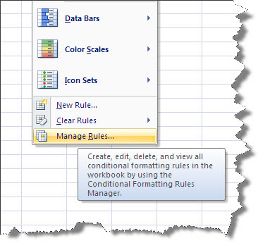
Go to Manage rules in the menu
Then select the rule from the list
This list allows you to manage the following
- The certain rule you can view all the rules in the worksheet, in another sheet, or in the selection
- Applies to, allows you to change the cells that are affected in this case =$B$4:$E$8

- If you wish to change this to the entire row 3 to 8 you would write =$3:$8
- Stop if True, and stop testing for other rules.
- Delete, add new, or move rule Up/Down (makes sense with point 3 - above)
